How To Calculate The Average In Excel (By Hand) Or Create A Formula For Average Explained
In this video we go over 2 different ways to calculate the average or create a formula to calculate the average in excel. We go step by step through the process for both ways
Transcript/notes
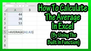
In this excel spreadsheet we have values in cells A1 thru A3, and let’s say that we want to find the average of these values and put the answer in cell C2.
There are 2 main ways to do this, by creating our own formula or by using the built in excel function for average. We are going to do this by creating our own formula in this video, and I am going to show you 2 ways to this by hand, so to speak.
For the first way, we start by left clicking on cell C2 so it is highlighted then we type in an equals sign, Next we type in an open parenthesis, then we left click on the first cell that will be part of the average calculation cell A1. Next we type in a plus or addition sign. Then we left click on the next cell we want as part of the average cell A2, then another addition sign, then we left click on the last cell to be part of the average, cell A3.
Next we type in a closed parenthesis. Now we type in a forward slash, which is the division sign in excel, then we type in the number of numbers being used to calculate the average, which in this case is 3. And we hit the enter key and we have our answer of 45.
Now for the second way. We are going to put the answer in cell C4, so, we start by left clicking on cell C4 so it is highlighted then, as before, we type in an equals sign. Here is where the difference begins. We type in an S, and a drop down box appears. We are going to scroll down in the box to the sum function you see here, and left double click on it.
Now, you see, in our answer cell sum then an open parenthesis, this is asking us to put some cell locations in here. For this, we are going to go to the first cell in our little data set, cell A1, and left click and hold, and then drag down to the last cell in our set, cell A3, then release the left click and hold.
From here, type in a closed parenthesis. Next, we type in a forward slash, or division sign, and then we are going to type in the letter C, and again a drop down box appears. We are going to scroll down the box to the word count, and left double click on it. Now, in our answer cell we have the word count then an open parenthesis, this is asking us to put some cell locations in here. As we did with the sum a moment ago, we are going to go to the first cell in our little data set, cell A1, and left click and hold, and then drag down to the last cell in our set, cell A3, then release the left click and hold. And next, we type in a closed parenthesis, then hit the enter key, and we have our answer again of 45.
This will also work if your values are all in the same row, as you see in this example.
Chapters/Timestamps
0:00 Example set up
0:15 How to calculate the average (method 1)
0:57 How to use sum function and count function to calculate the average


