Lookup the Last Value in a Column or Row in Excel - Get the Value in the Last Non-Empty Cell
In this video, I will show you how to lookup the value in the last non-empty cell in a row or column in Excel. You can use the LOOKUP function to get the last value.
First, create a formula to check whether the cell is empty or not. The formula returns an array that contains TRUE or FALSE values. If the value is TRUE, the cell is not empty. If the value is FALSE, the cell is empty. In the next column, apply the double negative method to convert boolean values into numeric values. If the value is one, the cell is non-empty. In the case of zero, the cell is empty. Modify the formula and use a division.
When you divide one by 1, you get 1. When you divide one by 0, you get a division-by-zero error. So, this array contains 1s. or errors. If the value is one, the cell is non-empty, and the errors correspond to empty cells. Type the LOOKUP function. The first argument is 2. Since two is greater than any possible value returned by the array. The second argument is the lookup vector. The array contains ones for non-empty cells. Or errors for empty cells. The last argument is a result vector, which is the range. Now, we have the value from the last non-empty cell in a range. Use the same method to get the last non-empty cell in a row.
Download DataFX free add-in:
https://exceldashboardschool.com/free...
Chapters:
00:00 Intro
00:08 Lookup the Last Value in a Column or Row - Find the Last Non-Empty Cell
🎓 LEARN MORE in my Excel tutorials: https://excelkid.com/
🔔 SUBSCRIBE if you’d like more tips and tutorials like this.
🎁 SHARE this video and spread the Excel love.
Or if you are in a hurry, please click the 👍
#excel #exceltips #exceltutorial

![Complete online adult ballet center [30 minutes]](https://images.videosashka.com/watch/IgZEpRMQ-cE)