Top 10 Microsoft Excel Tips & Tricks #4

Опубликовано: 09 Май 2025
на канале: Rabi Gurung

384

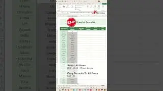
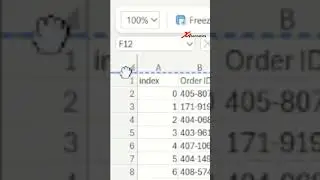
Tip 32 - Insert a Blank Row after Every Row in Excel
Learn how to insert blank row after every row in Excel.
Here are the steps.
1) Select second record
2) Hold Ctrl key and select every row one at a time.
3) Right-click on any selected row
4) Select Insert from context menu

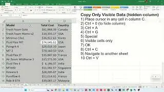
Tip 33 - Unstack Data from one Column to Multiple Columns - Clean Up Mixed Case Text
Learn how to unstack data from one column to multiple columns.
Here are the steps.
Populate Data
1) Select the whole stacked dataset.
2) Ctrl + C
3) Select first cell in next column
4) Ctrl + V
5) Select first cell in column
6) Ctrl + - (minus)
7) Shift cell up
8) OK
Filtering & Remove Rows
9) Data --- Filter
10) Filter first column "Sort Z to A"
11) Delete rows of data that is not suppose to be in the column.

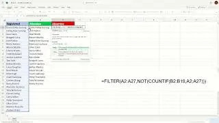
Tip 34 - 3 Ways To Check Spelling
Learn all the 3 ways to check spelling in your workbook.
Spell checking is essential to make the document look professional.
There are 3 ways to access spell checks.
1) Using hotkey F7
2) Using tabs. Review --- Spelling
3) Using Toolbar. Customize Quick Access Toolbar and enable Spelling. Click on Spelling icon.

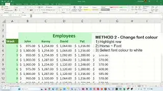
Tip 35 - Why you should avoid merging cells
Learn all about why you should avoid merging cells. I mean why you should never merge cells in excel. Seriously!
Here are the steps outlined in this video.
1) Select row of cells
2) Ctrl + 1
3) Alignment tab
4) In Horizontal pulldown menu, select "Center Across Selection"
5) OK
6) Delete data from cells

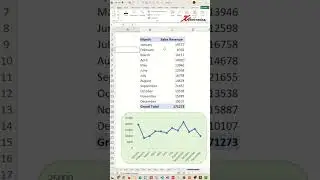
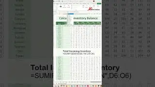
Tip 36 - How to Calculate Running Total or Cumulative Sum in Excel
Learn how to calculate running total or cumulative sum in Excel, fast and accurately.
1) Select transaction record
2) Ctrl + Q
3) Select Totals tab
4) Scroll to the right
5) Select "Running..." (yellow icon)

Tip 37 - Add a pop-up picture to a cell
Learn how to add a pop-up picture to a cell in Excel.
Here are the steps outlined in this video.
1) Right-click on cell you want to add pop.
2) Insert Comment
3) Remove text from popup (OPTIONAL)
4) Right-click just outside the pop border
5) Format Comment
6) Colours and Lines tab
7) Colours -- Fill Effects
8) Picture tab
9) Select Picture...
10) Select source of picture
11) Select your picture and Insert button
12) Lock picture aspect ratio (OPTIONAL)
13) OK
14) OK
15) Adjust size of popup

Tip 38 - Gantt Chart In Excel in under 5 seconds
Did you know that you can create a fully operational Gantt Chart in 5 click in Excel.
Here are the steps.
1) Launch Excel
2) New
3) Click on search bar and type the word gantt and press ENTER
4) Select the Gantt Chart template you like
5) Create

Tip 39 - How to Draw a Diagonal Line Through a Cell in Excel
Learn how to draw a diagonal line through a cell in Excel. This is especially good to show as a divider between row and column headers.
Here are the steps to draw the diagonal line
1) Select table corner cell.
2) Ctrl + 1
3) Border tab
4) Click on diagonal line.
5) OK
Here are the steps to add text to the header cell.
1) Select table corner cell.
2) Add a few spaces and enter row header text; "Month".
3) Alt + Enter to add new line
4) Enter column header text; "Name"
5) Press Enter when done.
Here are the steps to change font size of the header text
1) Double click "Month".
2) Change font size to 8.
3) Double click "Name".
4) Change font size to 8.

Tip 40 - WRAPROWS and WRAPCOLS function in Excel 365 - Excel Tips and Tricks
The WRAPCOLS and WRAPROWS Functions in Excel 365 "wraps" the provided row or column of values by rows after a specified number of elements to form a new array.
Raw data in one column (vertical table)
=WRAPROWS(G1:G90,5)
Raw data in one row (vertical table)
=WRAPROWS(G1:CR1,5)
(LONG) Flipping from one rows to one column data
=WRAPROWS(G1:CR1,1)
Raw data in one column (horizontal table)
=WRAPCOLS(B7:B96,5)
Raw data in one row (horizontal table)
=WRAPCOLS(B8:CM8,5)
Handling Errors with WRAPROWS
=WRAPROWS(A1:L1,5)
=WRAPROWS(A1:L1,5,"")
=WRAPROWS(A1:L1,5,"NA")

Tip 42 - How to identify or highlight expired or upcoming dates in Excel?
Learn how to identify or highlight expired and upcoming dates in Excel is important for a lot of retails stores from supermarkets to sale departments to computer parts store.
Today's Date
1) Select "Today's Date" cell.
2) Function
=today()
Days Left
1) Select first cell under "Days Left" column.
2) Function
=B6-$B$1
3) Apply to all rows.
Status
1) Select first cell under "Status" column.
2) Function
=IF(C6＜$B$2,"Expired",IF(C6＜=$B$3,"Warning","On Time"))
3) Apply to all rows.
Conditional Formatting Status Column
1) Select the "Status" column dataset.
2) Conditional Formatting
3) Highlight Cells Rules
4) Text that Contains...
5) Enter "Expired" and "Light Red Fill with Dark Red Text".
6) Steps 2 to 4.
7) Enter "Warning" and "Yellow Fill with Dark Yellow Text".
8) Steps 2 to 4.
9) Enter "On Time" and "Green Fill with Dark Green Text".

#tip #excel #microsoft #shorts #shortvideo #shortsvideo #howto #how #google